Computing flight curve
Reto Schmucki
29 March 2020
Generalized Abundance Index (1)
Here you we will use the rbms package to estimate a
regional flight curve for two different species, Maniola
jurtina and Polyommatus icarus. We will use a subset of
real data over 10 years, extracted from the eBMS database and generously
provided by our colleagues in France, the UK and the Netherlands. The
data have been anonymized and their spatial resolution limited to 1km
accuracy, but the count are real, including the noise.
The bms_workshop_data folder that can be downloaded here.
For this section, you will need to install and load the
rbms package available on GitHub with some explanation and
documentation available
here
## Loading required namespace: devtools## Using GitHub PAT from the git credential store.## Skipping install of 'rbms' from a github remote, the SHA1 (2016b299) has not changed since last install.
## Use `force = TRUE` to force installationIf you have difficulty to install the package directly, you can get the rbms.v_xxx.tar.gz file and install from file in R or RStudio.
##  Welcome to rbms, version 1.1.3
##  This package has been tested, but is still in active development and feedbacks are welcome
##  https://github.com/RetoSchmucki/rbms/issues
Here we will use the count and visit data.
Exploring data
Let’s first explore the data and what is in these two tables. Here we use the library DT to create an interactive table.
## Warning: package 'DT' was built under R version 4.4.3DT::datatable(b_count_sub[1:50, ], rownames = FALSE, filter = "top", options = list(pageLength = 5, scrollX = T))DT::datatable(m_visit_sub[1:50, ], rownames = FALSE, filter = "top", options = list(pageLength = 5, scrollX = T))## bms_id species_name
## <char> <char>
## 1: FRBMS Maniola jurtina
## 2: FRBMS Polyommatus icarus
## 3: NLBMS Polyommatus icarus
## 4: NLBMS Maniola jurtina
## 5: UKBMS Polyommatus icarus
## 6: UKBMS Maniola jurtina## [1] 2008 2009 2010 2011 2012 2013 2014 2015 2016 2017 2018Selecting species
The functions available in rbms package work on single
species and within one region. This way, the function can be run on
various cluster, in parallel or in for loops, but this is
your choice and here wi will run it for a single species in one
region.
- First let’s select a species
In the rbms package, you will find two example data set
with the required column names, these names are “hard coded” so they
need to be exactly the same in your data sets.
- Arrange data set name to fit the functions requirements
## change names in the data.table object
setnames(m_visit_sub, c("transect_id_serial", "visit_date"), c("SITE_ID", "DATE"))
names(m_visit_sub) <- toupper(names(m_visit_sub))

setnames(b_count_sub, c("transect_id_serial", "visit_date", "species_name"), c("SITE_ID", "DATE", "SPECIES"))
names(b_count_sub) <- toupper(names(b_count_sub))- Prepare a full time-series to align count, visit, monitoring and
flight curve estimate, using the function
ts_dwmy_table()- InitYear
- LastYear
- WeekDay1
- Define the monitoring season with the function
ts_monit_season()- ts_date
- StartMonth
- EndMonth
- StartDay
- EndDay
- CompltSeason
- Anchor
- AnchorLength
- AnchorLag
- TimeUnit (“d” or “w”)
ts_season <- rbms::ts_monit_season(ts_date,
                                   StartMonth = 4,
                                   EndMonth = 9,
                                   StartDay = 1,
                                   EndDay = NULL,
                                   CompltSeason = TRUE,
                                   Anchor = TRUE,
                                   AnchorLength = 2,
                                   AnchorLag = 2,
TimeUnit = "w")- Align the site visit in the region of interest with your monitoring season
MY_visit_region <- m_visit_sub[BMS_ID %in% region_bms, ]
ts_season_visit <- rbms::ts_monit_site(ts_season, MY_visit_region)- Align the butterfly counts recorded for the species and region of interest with your visit and monitoring season
Above, we already identified the species in the object
s_sp.
MY_count_region <- b_count_sub[BMS_ID %in% region_bms, ]
ts_season_count <- rbms::ts_monit_count_site(ts_season_visit, MY_count_region, sp = s_sp)- Estimate the flight curve for a species and region of interest,
using cubic spline smoother available in the
mgcvpackage.- ts_season_count
- NbrSample
- MinVisit
- MinOccur
- MinNbrSite
- MaxTrial
- GamFamily
- SpeedGam (logical)
- CompltSeason (logical)
- SelectYear
- TimeUnit (“d” or “w”)
ts_flight_curve <- rbms::flight_curve(ts_season_count,
                                            NbrSample = 500,
                                            MinVisit = 3,
                                            MinOccur = 2,
                                            MinNbrSite = 5,
                                            MaxTrial = 4,
                                            GamFamily = "nb",
                                            SpeedGam = FALSE,
                                            CompltSeason = TRUE,
                                            SelectYear = NULL,
                                            TimeUnit = "w"
                                            )

saveRDS(ts_flight_curve, file.path("bms_workshop_data", paste(gsub(" ", "_", s_sp), paste(region_bms, collapse="_"), "pheno.rds", sep = "_")))- Extract and plot the estimated phenology
ts_flight_curve <- readRDS(file.path("bms_workshop_data", paste(gsub(" ", "_", s_sp), paste(region_bms, collapse="_"), "pheno.rds", sep = "_")))

## explore the phenology
datatable(ts_flight_curve$pheno[1:370, .(SPECIES, M_YEAR, MONTH, trimWEEKNO, WEEK_SINCE, ANCHOR, NM)], rownames = FALSE, filter = "top", options = list(pageLength = 50, scrollX = T))
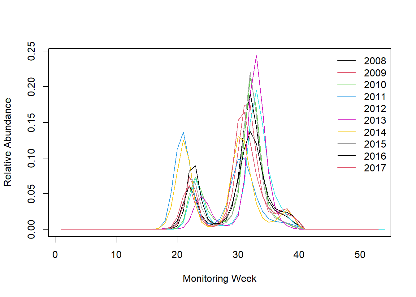
rbmsdoes not contain a plot method, so you have to make your own with your favourite tool.Bellow is example with plot in base R I am sure you can do better!
## Extract phenology part
pheno <- ts_flight_curve$pheno

## add the line of the first year
yr <- unique(pheno[order(M_YEAR), as.numeric(as.character(M_YEAR))])

if("trimWEEKNO" %in% names(pheno)){
  plot(pheno[M_YEAR == yr[1], trimWEEKNO], pheno[M_YEAR == yr[1], NM], type = 'l', ylim = c(0, max(pheno[, NM])), xlab = 'Monitoring Week', ylab = 'Relative Abundance')
} else {
  plot(pheno[M_YEAR == yr[1], trimDAYNO], pheno[M_YEAR == yr[1], NM], type = 'l', ylim = c(0, max(pheno[, NM])), xlab = 'Monitoring Day', ylab = 'Relative Abundance')

}

## add individual curves for additional years
if(length(yr) > 1) {
i <- 2
  for(y in yr[-1]){
    if("trimWEEKNO" %in% names(pheno)){
      points(pheno[M_YEAR == y , trimWEEKNO], pheno[M_YEAR == y, NM], type = 'l', col = i)
    } else {
      points(pheno[M_YEAR == y, trimDAYNO], pheno[M_YEAR == y, NM], type = 'l', col = i)
    }
    i <- i + 1
  }
}

## add legend
legend('topright', legend = c(yr), col = c(seq_along(c(yr))), lty = 1, bty = 'n')