Multi-species indicators
Emily Dennis
31 March 2020
Source trend functions required that you can download from this link.
Read in collated indices for two species and filter to one BMS
bms <- "UKBMS"
co_index <- rbind(readRDS("./bms_workshop_data/Maniola_jurtina_co_index_boot.rds"),
                  readRDS("./bms_workshop_data/Polyommatus_icarus_co_index_boot.rds"))
co_index <- co_index[BMS_ID == bms]
co_index
## BOOTi M_YEAR NSITE NSITE_OBS COL_INDEX BMS_ID SPECIES
## <num> <num> <int> <int> <num> <char> <char>
## 1: 0 2008 155 154 343.00258 UKBMS Maniola jurtina
## 2: 0 2009 216 215 316.96054 UKBMS Maniola jurtina
## 3: 0 2010 231 228 232.68168 UKBMS Maniola jurtina
## 4: 0 2011 232 228 273.07411 UKBMS Maniola jurtina
## 5: 0 2012 264 262 350.30579 UKBMS Maniola jurtina
## ---
## 10016: 500 2013 143 169 84.67527 UKBMS Polyommatus icarus
## 10017: 500 2014 150 163 57.17384 UKBMS Polyommatus icarus
## 10018: 500 2015 146 202 49.50536 UKBMS Polyommatus icarus
## 10019: 500 2016 139 158 26.61983 UKBMS Polyommatus icarus
## 10020: 500 2017 148 198 59.65347 UKBMS Polyommatus icarusConvert to log 10 collated indices (TRMOBS)
co_index[COL_INDEX > 0, LOGDENSITY:= log(COL_INDEX)/log(10)][, TRMOBS := LOGDENSITY - mean(LOGDENSITY) + 2, by = .(SPECIES, BOOTi)]
co_index
## BOOTi M_YEAR NSITE NSITE_OBS COL_INDEX BMS_ID SPECIES
## <num> <num> <int> <int> <num> <char> <char>
## 1: 0 2008 155 154 343.00258 UKBMS Maniola jurtina
## 2: 0 2009 216 215 316.96054 UKBMS Maniola jurtina
## 3: 0 2010 231 228 232.68168 UKBMS Maniola jurtina
## 4: 0 2011 232 228 273.07411 UKBMS Maniola jurtina
## 5: 0 2012 264 262 350.30579 UKBMS Maniola jurtina
## ---
## 10016: 500 2013 143 169 84.67527 UKBMS Polyommatus icarus
## 10017: 500 2014 150 163 57.17384 UKBMS Polyommatus icarus
## 10018: 500 2015 146 202 49.50536 UKBMS Polyommatus icarus
## 10019: 500 2016 139 158 26.61983 UKBMS Polyommatus icarus
## 10020: 500 2017 148 198 59.65347 UKBMS Polyommatus icarus
## LOGDENSITY TRMOBS
## <num> <num>
## 1: 2.535297 2.013024
## 2: 2.501005 1.978731
## 3: 2.366762 1.844488
## 4: 2.436281 1.914007
## 5: 2.544447 2.022173
## ---
## 10016: 1.927757 2.254929
## 10017: 1.757197 2.084370
## 10018: 1.694652 2.021825
## 10019: 1.425205 1.752378
## 10020: 1.775636 2.102809Next we calculate and plot the indicator, where the confidence interval is based on the bootstraps
First we generate the indicator for real data
##    year indicator ind_gam0    SMOOTH NSPECIES
## 1  2008  93.06434 63.45042 100.00000        2
## 2  2009 128.66868 78.32167 123.43759        2
## 3  2010 159.79842 79.71374 125.63153        2
## 4  2011  93.27168 64.26747 101.28769        2
## 5  2012  79.35512 63.13894  99.50909        2
## 6  2013 164.67445 87.10999 137.28827        2
## 7  2014 135.27982 95.79242 150.97207        2
## 8  2015 131.30396 79.97811 126.04818        2
## 9  2016  89.99077 79.85997 125.86200        2
## 10 2017 157.60336 89.84621 141.60064        2
Then generate an indicator for each bootstrap
##  num [1:10, 1:500] 59.9 73.6 75 60.9 61.7 ...
##  - attr(*, "dimnames")=List of 2
##   ..$ : NULL
## ..$ : chr [1:500] "1" "2" "3" "4" ...## 1 2 3 4 5
## [1,] 59.94336 63.03045 65.00111 63.97033 66.23381
## [2,] 73.55726 77.28879 79.18544 78.92274 83.27691
## [3,] 74.97925 78.57417 79.19096 80.36084 85.12711
## [4,] 60.88879 63.89199 61.36524 65.10461 68.43662
## [5,] 61.72164 62.75340 58.76827 62.95547 63.94505
## [6,] 87.33930 89.17058 84.65269 86.04877 87.39197
## [7,] 96.05617 99.77533 96.20685 95.91916 98.09845
## [8,] 79.92003 84.19464 82.31011 80.30745 81.79870
## [9,] 79.69771 82.81265 82.23267 80.10832 80.82010
## [10,] 89.77988 90.08617 90.71027 89.64004 89.36373Now we add a confidence interval to the indicator based on quantiles from the bootstrapped indicators
##    year indicator ind_gam0    SMOOTH NSPECIES LOWsmooth1 UPPsmooth1
## 1  2008  93.06434 63.45042 100.00000        2   88.14009   111.0803
## 2  2009 128.66868 78.32167 123.43759        2  112.91961   134.9132
## 3  2010 159.79842 79.71374 125.63153        2  114.83919   136.8903
## 4  2011  93.27168 64.26747 101.28769        2   92.73150   110.9626
## 5  2012  79.35512 63.13894  99.50909        2   89.62639   109.2745
## 6  2013 164.67445 87.10999 137.28827        2  125.17660   149.9729
## 7  2014 135.27982 95.79242 150.97207        2  140.38601   161.6547
## 8  2015 131.30396 79.97811 126.04818        2  116.72898   134.7303
## 9  2016  89.99077 79.85997 125.86200        2  120.03092   131.7026
## 10 2017 157.60336 89.84621 141.60064        2  139.70652   143.4271
Plot the indicator
ggplot(msi, aes(year, indicator))+
  theme(text = element_text(size = 14))+
  geom_ribbon(aes(ymin = LOWsmooth1, ymax = UPPsmooth1), alpha=.2, fill = "blue")+
  geom_point(color = "blue")+
  geom_line(aes(y = SMOOTH), color = "blue")+
  ylim(c(0, max(200,max(msi$UPPsmooth1))))+
  ggtitle(paste("Example indicator for", bms, "based on two species"))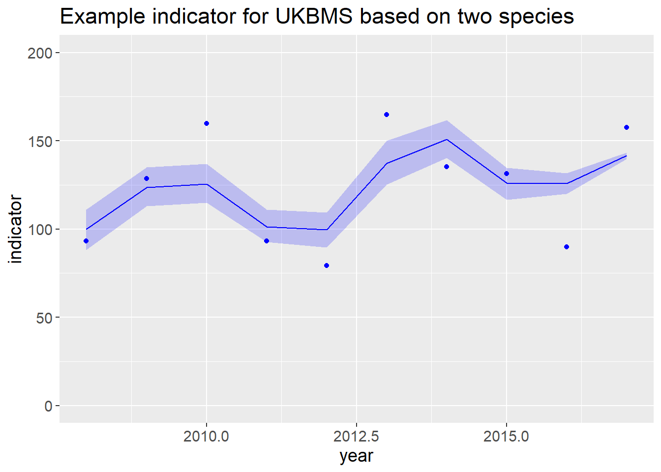
Calculate the indicator trend including confidence interval from the bootstraps
##   minyear maxyear nboot_lt  rate_lt rate_lt_low rate_lt_upp   pcn_lt pcn_lt_low
## 1    2008    2017      500 1.029534    1.017446     1.04204 29.94672   16.84273
##   pcn_lt_upp     TrendClass_lt
## 1   44.86399 Moderate increase