Mapping and extracting GIS information
Reto Schmucki
Mapping BMS sites
Working with spatially explicit data means that you can link them to various other environmental data sets. This also allow you to explore your data points visually and get a glimpse of there distribution and geographical context. In this short tutorial, we will explore how to generate spatial object from your BMS site data, using the R package sf, a powerful tool for geospatial computation in R.
In this session, you will:
- read csv file with data.table
- convert coordinates in spatial object using sf
- read raster file with the raster package
- produce a map with rasterVis and tmap
- extract value from raster using a vector object
You will need to load the following R packages and the data found in
the bms_workshop_data folder that can be
downloaded
here. Once you have downloaded the data, unzip the folder and add
the data in your R project directory, your current R working directory,
or set your working directly accordingly setwd().
## Linking to GEOS 3.12.1, GDAL 3.8.4, PROJ 9.3.1; sf_use_s2() is TRUE## terra 1.7.71##
## Attaching package: 'terra'## The following object is masked from 'package:data.table':
##
## shift## Warning: package 'tmap' was built under R version 4.4.2## Warning: package 'mapview' was built under R version 4.4.2All data are stored in rds format, this format is highly
efficient for storing R object, but you could also have them in any
other format. To load .rds data, we use the function
readRDS()
b_count_sub <- readRDS("bms_workshop_data/work_count.rds")
m_visit_sub <- readRDS("bms_workshop_data/work_visit.rds")
m_site_sub <- readRDS("bms_workshop_data/work_site.rds")
For this session, we will also upload a raster file with Bioclimate
Regions provided by
Metzger
et al. 2013 (see licence). tje raster file is
provided in .grd format and can be read into R with the
raster() function from the raster package. Together with
the raster file with the Bioclimate Regions, you can load the
classification available in a .csv and can be loaded with
data.table. To subset the data from the eBMS database, I
used a bounding box that can be loaded in R with the package
sf.
Mapping
bcz <- terra::rast("bms_workshop_data/metzger_bcz_genz3.grd")
bb <- sf::st_read("bms_workshop_data/bbox.shp")
bcz_class <- data.table::fread("bms_workshop_data/GEnS_v3_classification.csv")
First we will produce a spatial object for the points corresponding
to the BMS transects in the m_site_sub object (where “m” stands for
monitoring). Using the sf function st_as_sf() you can build
points from longitude/latitude coordinates and CRS=3035 as we use the
standard ETRS89-extended/LAEA Europe as projection
system EPGS:3035. You can have a
quick look at the points on a map with the function
mapview() from the R package mapview. This will open a
window in your browser with an interactive map of your points.
## sf transect location
site_sf <- sf::st_as_sf(m_site_sub, coords = c("transect_lon_1km", "transect_lat_1km"), crs = 3035)
mapview::mapview(site_sf)
Trick: you can extract a bounding box with the function draw() from terra package and build a corresponding polygon with the function st_as_sfc() from sf package.
st_as_sfc(st_bbox(terra::draw(), crs = st_crs(4326)))
Another option is to use the package tmap to produce “better looking
map”, but also much slower. For raster you will the function
tm_raster() and add other layers using the same principle
as in ggplot. Obviously, producing good looking and informative maps is
an art and you can spend ages working on them to get beautiful
results.
## adjust projection to 4326 for both the points an the bounding box objects.
site_sf_4326 <- st_transform(site_sf, 4326)
bb_4326 <- st_transform(bb, 4326)

## plot point on raster using tmap
tm_layout(frame = FALSE) +
tm_shape(bcz) +
  tm_raster(
    col.legend = tm_legend(title = "Bioclimate"),
    col.scale = tm_scale_categorical(values = 'viridis'),
    col_alpha = 1
    ) +
tm_shape(st_geometry(site_sf_4326)) +
tm_dots(fill = "orange", col="orange",  size = 0.1, shape = 20) +
tm_shape(st_geometry(bb_4326)) +
  tm_borders(
      lty = 2,
      col= 'magenta',
      lwd=2)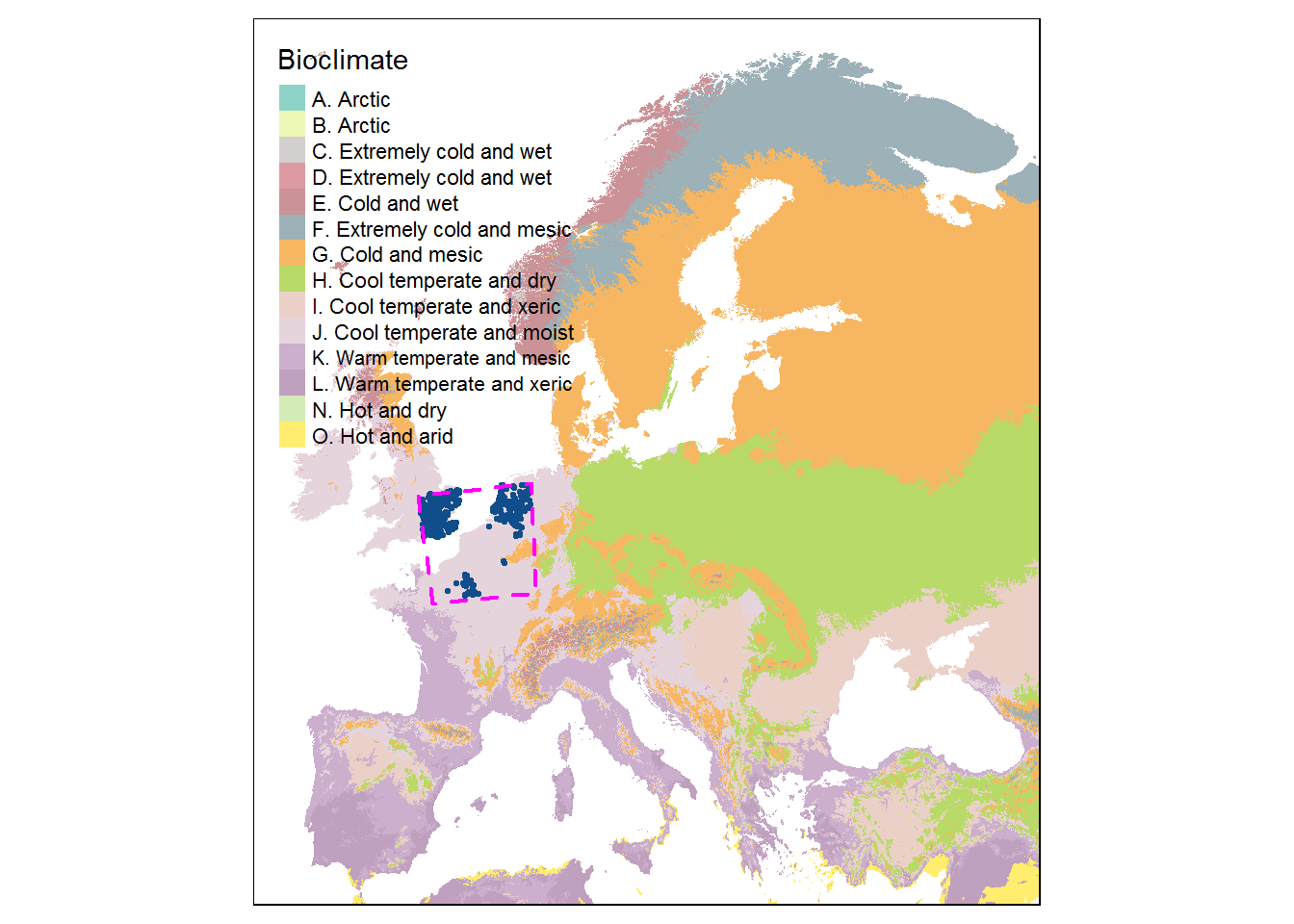
Extracting spatial information
Using the simple feature object produced previously from the site
data coordinates, you can now extract information from the Biogeographic
Region raster layer, using the function extract(). These
values can then be appended to your site data set using the
merge() method from the data.table package or your
favourite tidy tool.
site_dt <- data.table(sf::st_drop_geometry(site_sf_4326))
site_sf_4326 <- st_transform(site_sf_4326, crs = crs(bcz))
site_dt$GEnZ_seq <- as.integer(terra::extract(bcz, site_sf_4326, exact = TRUE)$Bioclimate)
site_dt <- merge(site_dt,
                unique(bcz_class[, .(GEnZ_seq, GEnZname)]),
                by = "GEnZ_seq",
                all.x=TRUE)
Exploring results
You can have a look at the result using below, with an interactive map to explore what just happened.