Calculating species trends
Emily Dennis
31 March 2020
Source trend functions required that you can download from this link.
Read in collated indices for species and BMS of interest
# Specify the species - note the underscore
spp <- "Maniola_jurtina"
# Specify the BMS
bms <- "UKBMS"
# Read in the bootstrapped collated indices
co_index <- readRDS(paste0("./bms_workshop_data/", spp, "_co_index_boot.rds"))
# Filter to a single BMS to focus upon
co_index <- co_index[BMS_ID == bms]
co_index
## BOOTi M_YEAR NSITE NSITE_OBS COL_INDEX BMS_ID SPECIES
## <num> <num> <int> <int> <num> <char> <char>
## 1: 0 2008 155 154 343.0026 UKBMS Maniola jurtina
## 2: 0 2009 216 215 316.9605 UKBMS Maniola jurtina
## 3: 0 2010 231 228 232.6817 UKBMS Maniola jurtina
## 4: 0 2011 232 228 273.0741 UKBMS Maniola jurtina
## 5: 0 2012 264 262 350.3058 UKBMS Maniola jurtina
## ---
## 5006: 500 2013 159 259 421.1923 UKBMS Maniola jurtina
## 5007: 500 2014 173 284 358.3261 UKBMS Maniola jurtina
## 5008: 500 2015 158 254 350.4547 UKBMS Maniola jurtina
## 5009: 500 2016 161 261 308.2660 UKBMS Maniola jurtina
## 5010: 500 2017 148 233 471.5391 UKBMS Maniola jurtinaConvert to log 10 collated indices (TRMOBS)
## Only use COL_INDEX larger then 0 for calculation or logdensity and trmobs
co_index[COL_INDEX > 0, LOGDENSITY:= log(COL_INDEX)/log(10)][, TRMOBS := LOGDENSITY - mean(LOGDENSITY) + 2, by = .(BOOTi)]
co_index
## BOOTi M_YEAR NSITE NSITE_OBS COL_INDEX BMS_ID SPECIES LOGDENSITY
## <num> <num> <int> <int> <num> <char> <char> <num>
## 1: 0 2008 155 154 343.0026 UKBMS Maniola jurtina 2.535297
## 2: 0 2009 216 215 316.9605 UKBMS Maniola jurtina 2.501005
## 3: 0 2010 231 228 232.6817 UKBMS Maniola jurtina 2.366762
## 4: 0 2011 232 228 273.0741 UKBMS Maniola jurtina 2.436281
## 5: 0 2012 264 262 350.3058 UKBMS Maniola jurtina 2.544447
## ---
## 5006: 500 2013 159 259 421.1923 UKBMS Maniola jurtina 2.624480
## 5007: 500 2014 173 284 358.3261 UKBMS Maniola jurtina 2.554278
## 5008: 500 2015 158 254 350.4547 UKBMS Maniola jurtina 2.544632
## 5009: 500 2016 161 261 308.2660 UKBMS Maniola jurtina 2.488926
## 5010: 500 2017 148 233 471.5391 UKBMS Maniola jurtina 2.673518
## TRMOBS
## <num>
## 1: 2.013024
## 2: 1.978731
## 3: 1.844488
## 4: 1.914007
## 5: 2.022173
## ---
## 5006: 2.094971
## 5007: 2.024769
## 5008: 2.015123
## 5009: 1.959416
## 5010: 2.144008Estimate and classify species trends with a confidence interval based on the bootstraps
## data_from data_to data_nyears minyear maxyear n nboot_lt rate_lt rate_lt_low
## 0 2008 2017 10 2008 2017 10 500 1.03176 1.018995
## rate_lt_upp pcn_lt TrendClass_lt
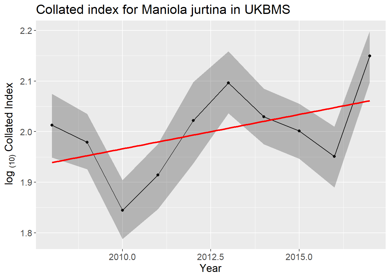
## 0 1.044679 32.49766 Moderate increasePlot the species log collated index with bootstrapped 95% confidence interval and linear trend line (in red)
# Calculate mean log index for original data
co_index0_mean <- mean(co_index[BOOTi == 0]$LOGDENSITY, na.rm = TRUE)
# Derive interval from quantiles
co_index_ci <- merge(co_index[BOOTi == 0, .(M_YEAR, TRMOBS, BMS_ID)],
                        co_index[BOOTi != 0, .(
                          LOWER = quantile(LOGDENSITY - co_index0_mean + 2, 0.025, na.rm = TRUE),
                          UPPER = quantile(LOGDENSITY - co_index0_mean + 2, 0.975, na.rm = TRUE)),
                          by = .(BMS_ID, M_YEAR)],
                        by=c("BMS_ID","M_YEAR"))


ggplot(co_index_ci, aes(M_YEAR, TRMOBS))+
  theme(text = element_text(size = 14))+
  geom_line()+
  geom_point()+
  geom_ribbon(aes(ymin = LOWER, ymax = UPPER), alpha = .3)+
  geom_smooth(method="lm", se=FALSE, color="red")+
  xlab("Year")+ylab(expression('log '['(10)']*' Collated Index'))+
  ggtitle(paste("Collated index for", gsub("_", " ", spp), "in", bms))
## `geom_smooth()` using formula = 'y ~ x'