Computing site and collated indices
Reto Schmucki
29 March 2020
Generalized Abundance Index (2)
After having successfully computed estimates of the regional flight curve, you can now use this information together with your count data to estimate a total number of butterfly per monitoring site over a season. This will provide you with an estimated abundance for each site that can be used to compute a collated index over the entire regions or a group of sites.
For this task, we will used the flight curve computed earlier and the
impute_count, site_index and finally
collated_index functions available in rbms
package
Here we will use the count and visit data.
# s_sp <- "Maniola jurtina"
s_sp <- "Polyommatus icarus"
region_bms <- c("NLBMS", "FRBMS")

b_count_sub <- readRDS("bms_workshop_data/work_count.rds")
m_visit_sub <- readRDS("bms_workshop_data/work_visit.rds")

setnames(m_visit_sub, c("transect_id_serial", "visit_date"), c("SITE_ID", "DATE"))
names(m_visit_sub) <- toupper(names(m_visit_sub))

setnames(b_count_sub, c("transect_id_serial", "visit_date", "species_name"), c("SITE_ID", "DATE", "SPECIES"))
names(b_count_sub) <- toupper(names(b_count_sub))

ts_date <- rbms::ts_dwmy_table(InitYear = 2008,
                               LastYear = 2017,
                               WeekDay1 = "monday")

ts_season <- rbms::ts_monit_season(ts_date,
                                   StartMonth = 4,
                                   EndMonth = 9,
                                   StartDay = 1,
                                   EndDay = NULL,
                                   CompltSeason = TRUE,
                                   Anchor = TRUE,
                                   AnchorLength = 2,
                                   AnchorLag = 2,
                                   TimeUnit = "w")

MY_visit_region <- m_visit_sub[BMS_ID %in% region_bms, ]
ts_season_visit <- rbms::ts_monit_site(MY_visit_region, ts_season)
## Warning in rbms::ts_monit_site(MY_visit_region, ts_season): We have changed the
## order of the input arguments, with ts_seaon now in first place, before m_visit.MY_count_region <- b_count_sub[BMS_ID %in% region_bms, ]
ts_season_count <- rbms::ts_monit_count_site(ts_season_visit, MY_count_region, sp = s_sp)
# ts_flight_curve <- rbms::flight_curve(ts_season_count,
# NbrSample = 500,
# MinVisit = 3,
# MinOccur = 2,
# MinNbrSite = 5,
# MaxTrial = 4,
# GamFamily = "nb",
# SpeedGam = FALSE,
# CompltSeason = TRUE,
# SelectYear = NULL,
# TimeUnit = "w"
# )
ts_flight_curve <- readRDS(file.path("bms_workshop_data", paste(gsub(" ", "_", s_sp), paste(region_bms, collapse="_"), "pheno.rds", sep = "_")))
pheno <- ts_flight_curve$phenoImpute & Site index
With the phenology and the observed counts, you can now calculate the values for missing weekly counts and appropriately calculate the abundance index for the entire monitoring season.
Note that until now (31/03/2025) the function “impute_count()” calculates the count with an arithmetic approach and not with the Generalised Linear Model with offset proposed in Schmucki et al. 2016. This was implemented for reasons of efficiency. However, the GLM with offset appears to be more robust in some cases, so this method will be reintegrated into this function in the future.
impt_counts <- rbms::impute_count(ts_season_count = ts_season_count,
                                  ts_flight_curve = pheno,
                                  YearLimit = NULL,
                                  TimeUnit = "w")

sindex <- rbms::site_index(butterfly_count = impt_counts, MinFC = 0.10)

saveRDS(sindex, file.path("bms_workshop_data", paste( gsub(" ", "_", s_sp), paste(region_bms, collapse="_"), "sindex.rds", sep="_")))
Collated index
Now that we have all each site index, we can collate them together to
estimate annual abundance indices for the wider region, using the
collated_index function in rbms. For this
example, we will focus on the sites monitored in the Netherlands (NLBMS)
and compute a collated index for Polyommatus icarus accross the
site monitored in that region over the 10-year period.
bms_id <- "NLBMS"

sindex <- readRDS(file.path("bms_workshop_data", paste( gsub(" ", "_", s_sp), paste(region_bms, collapse="_"), "sindex.rds", sep="_")))

sindex[substr(SITE_ID, 1, 5) == bms_id, ]
## Key: <M_YEAR, SITE_ID>
## SPECIES SITE_ID M_YEAR TOTAL_NM SINDEX
## <char> <char> <int> <num> <num>
## 1: Polyommatus icarus NLBMS.1 2008 0.38452 88.421929
## 2: Polyommatus icarus NLBMS.10 2008 0.71276 0.000000
## 3: Polyommatus icarus NLBMS.100 2008 0.41002 12.194527
## 4: Polyommatus icarus NLBMS.11 2008 0.70476 12.770305
## 5: Polyommatus icarus NLBMS.12 2008 0.77742 1.286306
## ---
## 2514: Polyommatus icarus NLBMS.94 2017 0.37326 8.037293
## 2515: Polyommatus icarus NLBMS.95 2017 0.44745 0.000000
## 2516: Polyommatus icarus NLBMS.96 2017 0.68085 0.000000
## 2517: Polyommatus icarus NLBMS.97 2017 0.74649 20.094040
## 2518: Polyommatus icarus NLBMS.98 2017 0.50655 7.896555co_index <- collated_index(data = sindex[substr(SITE_ID, 1, 5) == bms_id, ],
s_sp = s_sp,
sindex_value = "SINDEX",
glm_weights = TRUE,
rm_zero = TRUE)
co_index$col_index## Key: <M_YEAR>
## BOOTi M_YEAR NSITE NSITE_B NSITE_OBS COL_INDEX
## <num> <num> <int> <int> <int> <num>
## 1: 0 2008 203 203 137 23.25839
## 2: 0 2009 224 224 187 70.44026
## 3: 0 2010 236 236 191 51.13282
## 4: 0 2011 261 261 194 26.24425
## 5: 0 2012 277 277 189 23.85835
## 6: 0 2013 283 283 233 68.84266
## 7: 0 2014 277 277 224 46.76059
## 8: 0 2015 275 275 220 34.31891
## 9: 0 2016 257 257 192 26.03402
## 10: 0 2017 225 225 171 39.29854Bootstrap CI
With this sample of site indices, we can compute the collated indices
for multiple combination of sites. Using a bootstrap approach, we can
now estimate the confidence interval around the estimated collated
index, using the variation observed between monitoring sites. First we
randomly draw n bootstrap samples, using the function
boot_sample. This function sample with replacement from a
the pool of all sites available. Because sampling is done with
replacement, site can occur twice in a specific bootstrap sample and it
will be treated as two independent sites (realisations). Here we use a
500 bootstrap, with set.seed() sake of cpu time and repeatability, but
you should aim for 1000 sample and more and remove the set.seed() in the
random number generator to generate different samples between runs.
Note that we set “glm_weights = TRUE” in the “collated_index()” function. If you set this argument to “TRUE”, the function will use the portion of the flight curve sampled as the weight in the model. This means that poorly informed indices (site with few visits or with visits outside the flight curve) have less influence on the collated index than those that cover a larger proportion of the flight curve.
bms_id <- "NLBMS"
set.seed(125361)

bootsample <- rbms::boot_sample(sindex[substr(SITE_ID, 1, 5) == bms_id, ], boot_n = 500)
co_index <- list()

## for progression bar, uncomment the following
pb <- txtProgressBar(min = 0, max = dim(bootsample$boot_ind)[1], initial = 0, char = "*",  style = 3)

for (i in c(0, seq_len(dim(bootsample$boot_ind)[1]))) {
    co_index[[i + 1]] <- rbms::collated_index(data = sindex[substr(SITE_ID, 1, 5) == bms_id, ],
                                              s_sp = s_sp,
                                              sindex_value = "SINDEX",
                                              bootID = i,
                                              boot_ind = bootsample,
                                              glm_weights = TRUE,
                                              rm_zero = TRUE)

    ## for progression bar, uncomment the following
    setTxtProgressBar(pb, i)
}

## collate and append all the result in a data.table format
co_index <- rbindlist(lapply(co_index, FUN = "[[", "col_index"))
co_index$BMS_ID <- bms_id
co_index$SPECIES <- s_sp

co_index_boot <- co_index
saveRDS(co_index_boot, file.path("bms_workshop_data", paste( gsub(" ", "_", s_sp), bms_id, "co_index_boot.rds", sep="_")))
Figure with CI
Now that you have a collated index, and a series bootstrapped collated indices, you can compute a 95% Confidence Interval around your index and construct a figure to illustrate the temporal trend resulting from the annual indices. Here we will rescale and present the indices on a log(index)/log(10) scale. Confidence interval are computed using the 0.025 and 0.975 quantile from the n bootstrap sample.
bms_id <- "NLBMS"

co_index_boot <- readRDS(file.path("bms_workshop_data", paste( gsub(" ", "_", s_sp), bms_id, "co_index_boot.rds", sep="_")))

boot0 <- co_index_boot[ , mean(COL_INDEX, na.rm=TRUE), by = M_YEAR]
boot0[, LOGDENSITY0 := log(V1) / log(10)]
boot0[, meanlog0 := mean(LOGDENSITY0)]

# Add mean of BOOTi == 0 (real data) to all data
boot_ests <- merge(co_index_boot, boot0[, .(M_YEAR, meanlog0)],
    by = c("M_YEAR")
    )

boot_ests[, LOGDENSITY := log(COL_INDEX) / log(10)]
boot_ests[, TRMOBSCI := LOGDENSITY - meanlog0 + 2]

boot_ests[, TRMOBSCILOW := quantile(TRMOBSCI, 0.025), by = M_YEAR]
boot_ests[, TRMOBSCIUPP := quantile(TRMOBSCI, 0.975), by = M_YEAR]

ylim_ <- c(min(floor(range(boot_ests[TRMOBSCI <= TRMOBSCIUPP & TRMOBSCI >= TRMOBSCILOW, TRMOBSCI]))),
           max(ceiling(range(boot_ests[TRMOBSCI <= TRMOBSCIUPP & TRMOBSCI >= TRMOBSCILOW, TRMOBSCI]))))

plot_col <- ggplot(data = boot_ests[TRMOBSCI <= TRMOBSCIUPP & TRMOBSCI >= TRMOBSCILOW, ], aes(x = M_YEAR, y = TRMOBSCI)) +
    geom_point(colour = "orange", alpha = 0.2) + ylim(ylim_) +
    geom_line(data = boot_ests[TRMOBSCI <= TRMOBSCIUPP & TRMOBSCI >= TRMOBSCILOW, median(TRMOBSCI, na.rm=TRUE), by = M_YEAR], aes(x = M_YEAR, y = V1), linewidth = 1, colour = "dodgerblue4") +
    geom_hline(yintercept = 2, linetype = "dashed", color = "grey50") +
    scale_x_continuous(minor_breaks = waiver(), limits = c(2005, 2020), breaks = seq(2005, 2020, by = 5)) +
    xlab("Year") + ylab("Abundance Incices (Log/Log(10))") +
    labs(subtitle = paste(s_sp, bms_id, sep = " "))

plot_col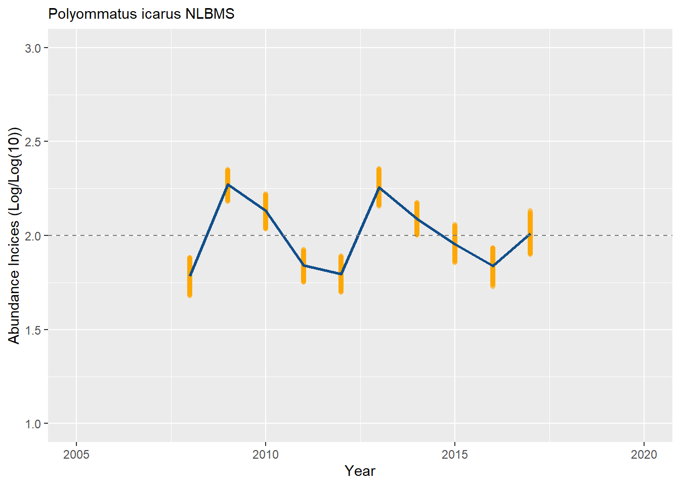
Now, let’s center the index on the first year instead (line #5 > “boot0[, first_year_log0 := boot0[order(M_YEAR), LOGDENSITY0][1]]”).
bms_id <- "NLBMS"

co_index_boot <- readRDS(file.path("bms_workshop_data", paste( gsub(" ", "_", s_sp), bms_id, "co_index_boot.rds", sep="_")))

boot0 <- co_index_boot[ , mean(COL_INDEX, na.rm=TRUE), by = M_YEAR]
boot0[, LOGDENSITY0 := log(V1) / log(10)]
boot0[, first_year_log0 := boot0[order(M_YEAR), LOGDENSITY0][1]]

# Add mean of BOOTi == 0 (real data) to all data
boot_ests <- merge(co_index_boot, boot0[, .(M_YEAR, first_year_log0)],
    by = c("M_YEAR")
    )

boot_ests[, LOGDENSITY := log(COL_INDEX) / log(10)]
boot_ests[, TRMOBSCI := LOGDENSITY - first_year_log0 + 2]

boot_ests[, TRMOBSCILOW := quantile(TRMOBSCI, 0.025), by = M_YEAR]
boot_ests[, TRMOBSCIUPP := quantile(TRMOBSCI, 0.975), by = M_YEAR]

ylim_ <- c(min(floor(range(boot_ests[TRMOBSCI <= TRMOBSCIUPP & TRMOBSCI >= TRMOBSCILOW, TRMOBSCI]))),
           max(ceiling(range(boot_ests[TRMOBSCI <= TRMOBSCIUPP & TRMOBSCI >= TRMOBSCILOW, TRMOBSCI]))))

plot_col <- ggplot(data = boot_ests[TRMOBSCI <= TRMOBSCIUPP & TRMOBSCI >= TRMOBSCILOW, ], aes(x = M_YEAR, y = TRMOBSCI)) +
    geom_point(colour = "orange", alpha = 0.2) + ylim(ylim_) +
    geom_line(data = boot_ests[TRMOBSCI <= TRMOBSCIUPP & TRMOBSCI >= TRMOBSCILOW, median(TRMOBSCI, na.rm=TRUE), by = M_YEAR], aes(x = M_YEAR, y = V1), linewidth = 1, colour = "dodgerblue4") +
    geom_hline(yintercept = 2, linetype = "dashed", color = "grey50") +
    scale_x_continuous(minor_breaks = waiver(), limits = c(2005, 2020), breaks = seq(2005, 2020, by = 5)) +
    xlab("Year") + ylab("Abundance Incices (Log/Log(10))") +
    labs(subtitle = paste(s_sp, bms_id, sep = " "))

plot_col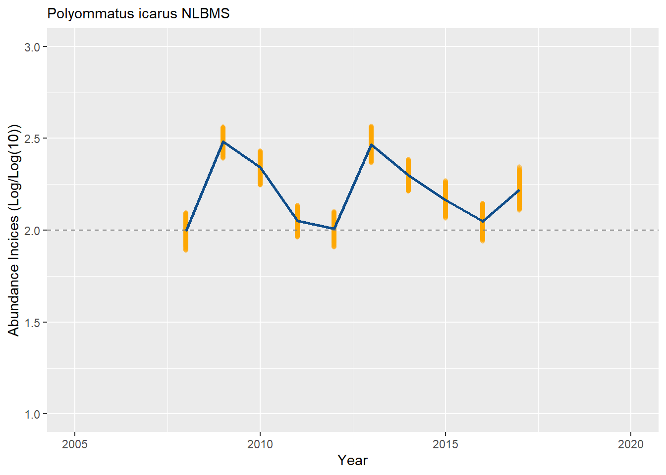
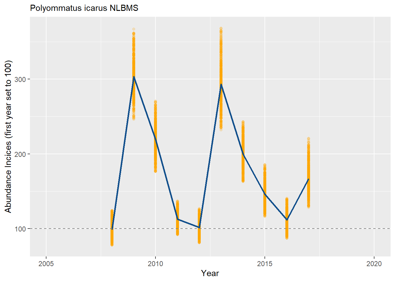
Now, let’s center the index on the first year and scale it to 100 instead of 2, using 10^2 = 100 (line #10 > “boot_ests[, TRMOBSCI := 10^(LOGDENSITY - first_year_log0 + 2)]”). Note that we have also changed the intercept to 100 in the figure. This may be easier to interpret as we start at 100 and have an increase or decrease relative to this baseline.
bms_id <- "NLBMS"

co_index_boot <- readRDS(file.path("bms_workshop_data", paste( gsub(" ", "_", s_sp), bms_id, "co_index_boot.rds", sep="_")))

boot0 <- co_index_boot[ , mean(COL_INDEX, na.rm=TRUE), by = M_YEAR]
boot0[, LOGDENSITY0 := log(V1) / log(10)]
boot0[, first_year_log0 := boot0[order(M_YEAR), LOGDENSITY0][1]]

# Add mean of BOOTi == 0 (real data) to all data
boot_ests <- merge(co_index_boot, boot0[, .(M_YEAR, first_year_log0)],
    by = c("M_YEAR")
    )

boot_ests[, LOGDENSITY := log(COL_INDEX) / log(10)]
boot_ests[, TRMOBSCI := 10^(LOGDENSITY - first_year_log0 + 2)]

boot_ests[, TRMOBSCILOW := quantile(TRMOBSCI, 0.025), by = M_YEAR]
boot_ests[, TRMOBSCIUPP := quantile(TRMOBSCI, 0.975), by = M_YEAR]

ylim_ <- c(min(floor(range(boot_ests[TRMOBSCI <= TRMOBSCIUPP & TRMOBSCI >= TRMOBSCILOW, TRMOBSCI]))),
           max(ceiling(range(boot_ests[TRMOBSCI <= TRMOBSCIUPP & TRMOBSCI >= TRMOBSCILOW, TRMOBSCI]))))

plot_col <- ggplot(data = boot_ests[TRMOBSCI <= TRMOBSCIUPP & TRMOBSCI >= TRMOBSCILOW, ], aes(x = M_YEAR, y = TRMOBSCI)) +
    geom_point(colour = "orange", alpha = 0.2) + ylim(ylim_) +
    geom_line(data = boot_ests[TRMOBSCI <= TRMOBSCIUPP & TRMOBSCI >= TRMOBSCILOW, median(TRMOBSCI, na.rm=TRUE), by = M_YEAR], aes(x = M_YEAR, y = V1), linewidth = 1, colour = "dodgerblue4") +
    geom_hline(yintercept = 100, linetype = "dashed", color = "grey50") +
    scale_x_continuous(minor_breaks = waiver(), limits = c(2005, 2020), breaks = seq(2005, 2020, by = 5)) +
    xlab("Year") + ylab("Abundance Incices (first year set to 100)") +
    labs(subtitle = paste(s_sp, bms_id, sep = " "))

plot_col